Machine learning · Web interface
NeuroVision (MRI)
Classifying MRI images into four classes with transfer learning.
Application screens
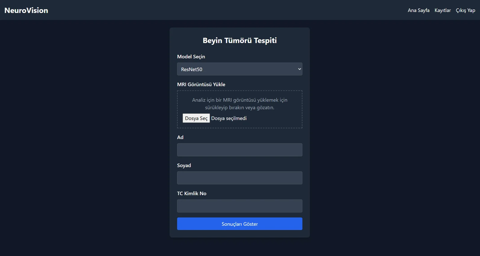
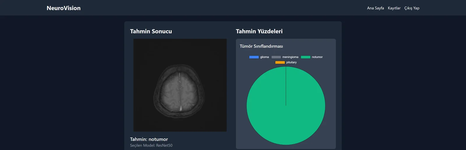
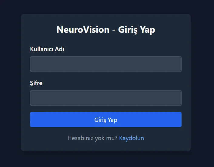
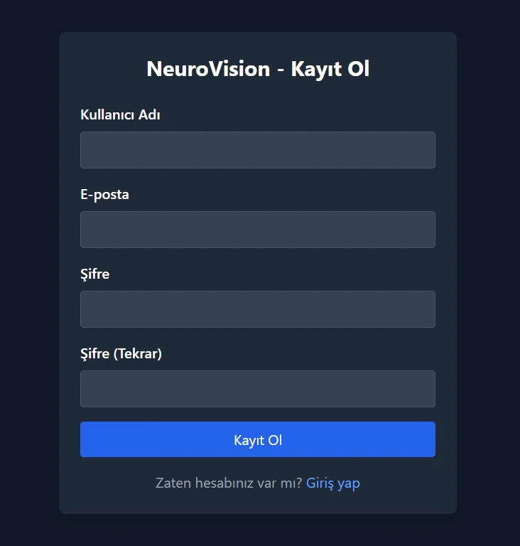
Home page1 / 4
Test results
| Model | Correct / Total | Accuracy |
|---|---|---|
| ResNet50 | 1368 / 1405 | 97.4% |
| ResNet101 | 1395 / 1405 | 99.3% |
Classes: glioma, meningioma, notumor (no tumor), pituitary.
What I built
Data
I combined the Training and Testing folders of Kaggle’s Brain Tumor MRI Dataset: 7,023 images, with 1,621 glioma, 1,645 meningioma, 2,000 notumor and 1,757 pituitary images. I randomly split them into 72% training, 8% validation and 20% test.
- 7,023 images
- 4 classes
- 72% / 8% / 20%
Preprocessing and augmentation
I resized images to 224×224×3 and one-hot encoded the labels. During training I used 40° rotation, 0.2 shifts/shear/zoom and horizontal flips, with nearest filling.
- 224×224×3
- One-hot
- ImageDataGenerator
Model setup
I froze the first 30 / 50 layers of ImageNet-weighted ResNet50 and ResNet101, leaving the remaining layers trainable. I added classification layers with GlobalAveragePooling2D, two dropout layers, 128 ReLU units and a four-class softmax output; dropout rates were 0.5 / 0.6 respectively.
- ImageNet
- 30 / 50 frozen
- Dropout 0.5 / 0.6
Training
I used Adam with learning rates of 0.001 / 0.0001 and batch sizes of 32 / 16. ModelCheckpoint, ReduceLROnPlateau and EarlyStopping were enabled; training stopped at epochs 18 / 36 against a 50-epoch limit. ResNet50 ran locally on a CPU, while ResNet101 ran on a Google Colab Tesla T4.
- Adam
- Batch 32 / 16
- 18 / 36 epochs
Evaluation
I compared both models on the same 1,405-image test set. Alongside accuracy and loss curves, I used confusion matrices, precision, recall and F1 to examine class-level errors.
- 1,405 test images
- Confusion matrix
- Precision / recall / F1
Web interface
I replaced the initial Flask prototype with a Django interface. The flow combines MRI upload and ResNet50/101 selection with the predicted class and class probabilities.
- Flask → Django
- Model selection
- Class probabilities
Model training
- MRI input224×224×3
- ResNet50 / ResNet101 · ImageNetFirst 30 / 50 layers: frozenRemaining layers: trainable
- GlobalAveragePooling2D
- Dropout · 0.5 / 0.6
- Dense 128 · ReLU
- Dropout · 0.5 / 0.6
- Dense 4 · softmax
- glioma / meningioma / notumor / pituitary
| Setting | ResNet50 | ResNet101 |
|---|---|---|
| Input | 224×224×3 | 224×224×3 |
| Pretraining | ImageNet | ImageNet |
| First frozen layers | 30 | 50 |
| Dropout (both layers) | 0.5 | 0.6 |
| Optimizer | Adam | Adam |
| Learning rate | 0.001 | 0.0001 |
| Loss | categorical_crossentropy | categorical_crossentropy |
| Batch size | 32 | 16 |
| Epoch limit | 50 | 50 |
| Stopped epoch | 18 | 36 |
| ModelCheckpoint | val_loss · save_best_only | val_loss · save_best_only |
| EarlyStopping patience | 5 | 7 |
| ReduceLROnPlateau patience | 3 | 5 |
| ReduceLROnPlateau factor / min_lr | 0.1 / 0.000001 | 0.1 / 0.000001 |
| Environment | Local CPU | Colab · Tesla T4 |
Results and analysis
Confusion matrices
ResNet50 misclassified 37 images in total, compared with 10 for ResNet101. The largest ResNet50 error was 18 meningioma images predicted as pituitary; another 5 meningioma images were labelled 'no tumor'. All 10 ResNet101 errors involve meningioma (meningioma being mistaken for another class, or another class being mistaken for meningioma); 31 of ResNet50's 37 errors involve meningioma. Meningioma is the hardest class for both models.
ResNet50 — confusion matrix
ResNet101 — confusion matrix
Class-level report
Meningioma recall (0.92) and pituitary precision (0.94) are the lowest values; both largely stem from the same error, misclassifying meningioma as pituitary. Recall for “no tumor” is 1.00 in the report’s two-decimal display (418/419).
ResNet50, test — classification report
Accuracy and loss curves
ResNet101 — accuracy
Training and validation accuracy converge around 99% after roughly epoch 10. No large separation is visible afterwards; this chart alone does not establish generalisation performance.
ResNet101 — loss
Training and validation loss fall rapidly after fluctuations in the first epochs. Both remain low after roughly epoch 10, with no sustained rise visible in validation loss.
ResNet50 — accuracy
Validation accuracy fluctuates initially and rises sharply around epoch 6. Near the end, training is around 99% and validation around 97%; this small gap alone does not prove overfitting. The chart’s “test” label refers to the notebook’s val_accuracy, the validation series.
ResNet50 — loss
Initial validation loss reaches roughly 450, making the vertical scale very wide. Later values are compressed near zero, so small late-epoch changes cannot be read reliably from this chart. The chart’s “test” label refers to the notebook’s val_loss, the validation series.
Data distribution
The four classes are reasonably close in size (1,621–2,000); glioma is the smallest and notumor the largest. The split chart shows 72% training, 8% validation and 20% test; the test class chart shows 310 / 326 / 419 / 350 images.
Data split — train 72%, validation 8%, test 20%
Test set class distribution
Data augmentation example
Training images received 40° rotation, 0.2 width/height shifts, shear and zoom, and horizontal flips. Empty areas used nearest filling; no additional augmented samples were generated for validation or test.
Data augmentation example
Key concepts
CNN (convolutional neural network)
It learns patterns by scanning an image with small filters: early layers capture edges and texture, deeper layers capture shapes and structures. ResNet50 and ResNet101 are the CNNs used in this project.
Pooling
Pooling makes a feature map smaller while preserving important information, reducing computation. Types include max pooling (the largest value in each window), average pooling (the window mean), and global average pooling (one number for each entire channel). This project used two types. In ResNet's first block, max pooling makes the image smaller while keeping the largest value in each region. Global average pooling was used after ResNet's final layer: it reduces each feature map to a single mean value, and the resulting numbers become inputs to the classification layers.
Teaching example: non-overlapping 2×2 windows, stride 2. Each colour connects a quadrant with its result.
Transfer learning and frozen layers
We froze the first layers of networks pretrained on ImageNet (30 in ResNet50, 50 in ResNet101), then trained the added classification layers and the remaining network layers on MRI data.
Limiting overfitting
We used data augmentation, dropout (0.5 / 0.6) and EarlyStopping to limit memorisation of the training data.
Evaluation metrics
We evaluated accuracy, precision, recall, F1 and confusion matrices. Rows represent true classes, columns predictions; diagonal entries are correct predictions. ResNet50 predicted 18 meningioma images as pituitary.
Technologies
Models and image processing
- Pythonapplication and training code
- TensorFlowmodel training and inference
- Keras (tf.keras)classification layers and training API
- NumPyarray operations
- scikit-learndata splitting and evaluation
- OpenCVimage loading and resizing
Web interface and records
- Djangoweb interface, sign-in and records
- Pillowuploaded image processing
- SQLitestoring Django records
Visualisation
- Matplotlibaccuracy, loss and distribution charts
- seabornconfusion matrix visualisation